Molecular neural network models with RDKit and Keras in Python

Esben Jannik Bjerrum/ December 6, 2016/ Blog, Cheminformatics, Machine Learning, Neural Network, RDkit/ 1 comments

Neural networks are interesting models underlying much of the newest AI applications and algorithms. Recent advances in training algorithms and GPU enabled code together with publicly available highly efficient libraries such as Google’s Tensorflow or Theano makes them highly interesting for modelling molecular data. Here I explore the high level Neural Network library for Python, Keras, which can interface for both Theano or Tenserflow for the underlying number crunching. Having a high level API in python for quickly defining the neural network architecture and training makes it fast to prototype the molecular data modelling. For this first model I use a solubility dataset I have used before: http://www.cheminformania.com/useful-information/wash-that-gold-modelling-solubility-with-molecular-fingerprints/
We start with some imports. I’ll need RDkit for molecular conversion and descriptor calculation, Pandas for loading and data management, Scikit-learn for standardisation and data set splitting as well as Keras for the neural network building and training.

from rdkit import Chem
from rdkit.Chem.EState import Fingerprinter
from rdkit.Chem import Descriptors
import pandas as pd
import numpy as np
from sklearn.preprocessing import StandardScaler
from sklearn import cross_validation
from keras.models import Sequential
from keras.layers import Dense, Activation
from keras.optimizers import SGD

The next couple of lines read the dataset into a Pandas dataframe object. The last 27 lines contains comments, so they are skipped. I want to use the E-state indices together with the molecular weight, so I define a function that calculates this. Afterwards its easy to add two new columns to the dataframes by applying functions to the existing column containing the molecules. First a column of RDkit mols are created from the column containing the SMILES strings, and afterwards the descriptor arrays are calculated.

#Read the data
data = pd.read_table('Solubility_data.smiles', sep=' ', skipfooter=27)
#Define a helper function to append the Molweight to the E-state indices
def fps_plus_mw(mol):
return np.append(Fingerprinter.FingerprintMol(mol)[0],Descriptors.MolWt(mol))
#Add some new columns
data['Mol'] = data['smiles'].apply(Chem.MolFromSmiles)
data['Descriptors'] = data['Mol'].apply(fps_plus_mw)

Unfortunately Scikit-learn can’t always use pandas dataframes, so a conversion to Numpy arrays are necessary. Standard scaling is applied and the dataset split into a train and test set.

#Convert to Numpy arrays
X = np.array(list(data['Descriptors']))
y = data['solubility'].values
#Scale X to unit variance and zero mean
st = StandardScaler()
X= st.fit_transform(X)
#Divide into train and test set
X_train, X_test, y_train, y_test = cross_validation.train_test_split(X, y, test_size=0.25, random_state=42)

Now the fun begins. Keras uses a base model object and adds the layers and activations as other objects in a sequential manner. The first layer must get an input dimensions matching the data, whereas the following can deduce their input size from the previous layer. Its a very simple model with a small hidden layer of 5 neurons with sigmoid activation. Larger networks will overfit, unless some form of regularization is put in place (such as early stopping or drop out). As the output values are continuous rather than class labels, the output dimension is a single neuron with a linear activation.

model = Sequential()
model.add(Dense(output_dim=5, input_dim=X.shape[1]))
model.add(Activation("sigmoid"))
model.add(Dense(output_dim=1))
model.add(Activation("linear"))

Before the  network can be trained using the Theano backend, the optimizer algorithm and the loss function need to be defined. The loss function is set for the usual mean squared error and the optimizer is stochastic gradient descent with a learning rate of 0.01 and a momentum of 0.9, using the Nesterov modification of the gradient.

model.compile(loss='mean_squared_error', optimizer=SGD(lr=0.01, momentum=0.9, nesterov=True))
history = model.fit(X_train, y_train, nb_epoch=500, batch_size=32)
y_pred = model.predict(X_test)
rms = (np.mean((y_test.reshape(-1,1) - y_pred)**2))**0.5
#s = np.std(y_test -y_pred)
print "Neural Network RMS", rms

 

.....
Epoch 499/500
983/983 [==============================] - 0s - loss: 0.2857
Epoch 500/500
983/983 [==============================] - 0s - loss: 0.2848
Neural Network RMS 0.855494851649

I was positively surprised by the fitting time of the network, even though I could only use CPU and not GPU on my laptop.
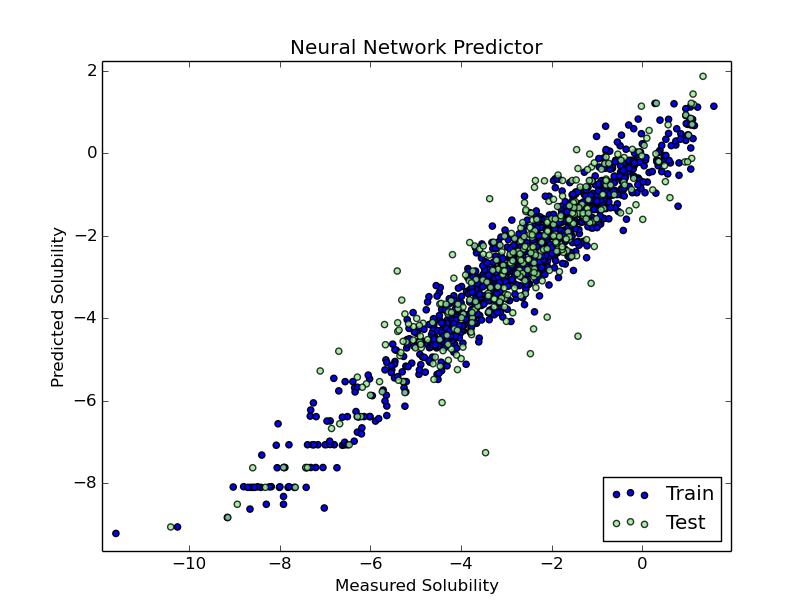
After fitting it was easy to predict the values of the test set and make a quick plot. RMS doesn’t seem so good, compared with previous models I’ve built, but this was meant as a fast test of Keras and Theano on an easy dataset.

import matplotlib.pyplot as plt
plt.scatter(y_train,model.predict(X_train), label = 'Train', c='blue')
plt.title('Neural Network Predictor')
plt.xlabel('Measured Solubility')
plt.ylabel('Predicted Solubility')
plt.scatter(y_test,model.predict(X_test),c='lightgreen', label='Test', alpha = 0.8)
plt.legend(loc=4)
plt.show()